数据库SQL总结

An introduction to join ordering

The development of the relational model heralded a big step forward for the world of databases. A few years later, SQL introduced a rich vocabulary for data manipulation: filters, projections, and—most importantly—the mighty join. Joins meant that analysts could construct new reports without having to interact with those eggheads in engineering, but more importantly, the existence of complex join queries meant that theoreticians had an interesting new NP-hard problem to fawn over for the next five decades.

关系模型的发展预示着数据库世界向前迈出了一大步。 几年后，SQL 引入了丰富的数据操作词汇：过滤器、投影，以及最重要的强大的连接。 连接意味着分析师可以构建新的报告，而无需与工程中的那些书呆子进行交互，但更重要的是，复杂连接查询的存在意味着理论家在接下来的 50 年里将面临一个有趣的新 NP 难题。

Ever since, the join has been the fundamental operation by which complex queries are constructed out of simpler “relations”. The declarative nature of SQL means that users do not generally specify how their query is to be executed—it’s the job of a separate component of the database called the optimizer to figure that out. Since joins are so prevalent in such queries, the optimizer must take special care to handle them intelligently. As we’ll see, this isn’t a trivial task.

从那时起，连接就成为了从更简单的“关系”构建复杂查询的基本操作。 SQL 的声明性本质意味着用户通常不会指定如何执行查询，而是数据库的一个单独组件（称为优化器）的工作来解决这个问题。 由于连接在此类查询中非常普遍，因此优化器必须特别小心以智能地处理它们。 正如我们将看到的，这不是一项简单的任务。

In this post, we’ll look at why join ordering is so important and develop a sense of how to think of the problem space. And then, in upcoming posts, we’ll begin discussing ways to implement a fast, reliable algorithm to produce good join orderings.

在这篇文章中，我们将了解为什么连接顺序如此重要，并培养如何思考问题空间的意识。 然后，在接下来的文章中，我们将开始讨论如何实现快速、可靠的算法来产生良好的连接顺序。

A Refresher on SQL and Joins

Let’s do a quick refresher in case you don’t work with SQL databases on a regular basis.

如果您不定期使用 SQL 数据库，让我们快速回顾一下。

A relation or table is basically a spreadsheet. Say we have the following relations describing a simple retailer:

关系或表基本上是一个电子表格。 假设我们有以下描述一个简单零售商的关系：

• customers
• products
• orders

The customers, or C relation looks something like this:

customer_id	customer_name	customer_location
1	Joseph	Norwalk, CA, USA
2	Adam	Gothenburg, Sweden
3	William	Stockholm, Sweden
4	Kevin	Raleigh, NC, USA

the products, or P relation looks like this:

product_id	product_location
123	Norwalk, CA, USA
789	Stockholm, Sweden
135	Toronto, ON, Canada

The orders, or O relation looks like this:

order_id	order_product_id	order_customer_id	order_active
1	123	3	false
2	789	1	true
3	135	2	true

The cross product of the two relations, written P×O, is a new relation which contains every pair of rows from the two input relations. Here’s what P×O looks like:

两个关系的叉积写为 P×O，是一个新关系，其中包含两个输入关系中的每对行。P×O 看起来像这样：

product_id	product_location	order_id	order_product_id	order_customer_id	order_active
123	Norwalk, CA, USA	1	123	3	false
123	Norwalk, CA, USA	2	789	1	true
123	Norwalk, CA, USA	3	135	2	true
789	Stockholm, Sweden	1	123	3	false
789	Stockholm, Sweden	2	789	1	true
789	Stockholm, Sweden	3	135	2	true
135	Toronto, ON, Canada	1	123	3	false
135	Toronto, ON, Canada	2	789	1	true
135	Toronto, ON, Canada	3	135	2	true

However, for most applications, this doesn’t have much meaning, which is where joins come into play.

然而，对于大多数应用程序来说，这没有多大意义，这就是连接发挥作用的地方。

A join is when we have a filter (or predicate) applied to the cross product of two relations. If we filter the above table to the rows where product_id = order_product_id, we say we’re “joining P and O on product_id = order_product_id“. The result looks like this:

连接是指我们将过滤器（或谓词）应用于两个关系的叉积。 如果我们将上表过滤到 product_id = order_product_id 的行，我们就说我们正在“在 product_id = order_product_id 上连接 P 和 O”。 结果如下：

product_id	product_location	order_id	order_product_id	order_customer_id	order_active
123	Norwalk, CA, USA	1	123	3	false
789	Stockholm, Sweden	2	789	1	true
135	Toronto, ON, Canada	3	135	2	true

Here we can see all of the orders that contained a given product.

在这里我们可以看到包含给定产品的所有订单。

We can then remove some of the columns from the output (this is called projection):

然后我们可以从输出中删除一些列（这称为投影）：

product_id	order_customer_id
123	3
789	1
135	2

This ends up with a relation describing the products various users ordered. Through pretty basic operations, we built up some non-trivial meaning. This is why joins are such a major part of most query languages (primarily SQL): they’re very conceptually simple (a predicate applied to the cross product) but can express fairly complex operations.

最终得到一个描述不同用户订购的产品的关系。 通过相当基本的操作，我们建立了一些不平凡的意义。 这就是为什么连接是大多数查询语言（主要是 SQL）的主要部分：它们在概念上非常简单（应用于叉积的谓词），但可以表达相当复杂的操作。

You might have observed that even though the size of the cross product was quite large (∣P∣×∣O∣), the final output was pretty small. Databases will exploit this fact to perform joins much more efficiently than by producing the entire cross product and then filtering it. This is part of why it’s often useful to think of a join as a single unit, rather than two composed operations.

您可能已经观察到，尽管叉积的大小非常大 (∣P∣×∣O∣)，但最终输出却非常小。 数据库将利用这一事实来比生成整个叉积然后过滤它更有效地执行连接。 这就是为什么将连接视为单个单元而不是两个组合操作通常很有用的部分原因。

Some Vocabulary 一些词汇

To make things easier to write, we’re going to introduce a little bit of notation.

为了使事情更容易编写，我们将引入一些符号。

We already saw that the cross product of A and B is written A×B. Filtering a relation R on a predicate p is written σ**p(R). That is, ��(�)σ**p(R) is the relation with every row of �R for which �p is true, for example, the rows where product_id = order_product_id. Thus a join of �A and �B on �p could be written ��(�×�)σ**p(A×B). Since we often like to think of joins as single cohesive units, we can also write this as �⋈��A⋈p**B.

The columns in a relation don’t need to have any particular order (we only care about their names), so we can take the cross product in any order. A×B=B×A, and further, A⋈pB*=B⋈*pA*. You might know this as the commutative property. Joins are commutative.

关系中的列不需要有任何特定的顺序（我们只关心它们的名称），因此我们可以按任何顺序进行叉积。 A×B=B×A，进而，A⋈pB*=B⋈*pA*。 您可能知道这是可交换属性。 连接是可交换的。

We can “pull up” a filter through a cross product: σ**p(A)×B=σ**p(A×B). It doesn’t matter if we do the filtering before or after the product is taken. Because of this, it sometimes makes sense to think of a sequence of joins as a sequence of cross products which we filter at the very end:

我们可以通过叉积“拉起”一个过滤器：σ**p(A)×B=σ**p(A×B)。 我们在产品服用之前或之后进行过滤并不重要。 因此，有时将连接序列视为我们在最后进行过滤的叉积序列是有意义的：

(A⋈p**B)⋈q**C=σ**q(σ**p(A×B)×C)=σ**p∧q(A×B×C)

Something that becomes clear when written in this form is that we can join A with B and then join the result of that with C, or we can join B with C and then join the result of that with A. The order in which we apply those joins doesn’t matter, as long as all the necessary filtering happens at some point. You might recognize this as the associative property. Joins are associative (with the asterisk that we need to pull up predicates where appropriate).

当以这种形式编写时，我们可以清楚地看到，我们可以将 A 与 B 连接，然后将其结果与 C 连接，或者我们可以将 B 与 C 连接，然后将其结果连接 与A。 只要所有必要的过滤在某个时刻发生，我们应用这些连接的顺序并不重要。 您可能会将其视为关联属性。 连接是关联的（带有星号，我们需要在适当的情况下提取谓词）。

Optimizing Joins

So we can perform our joins in any order we please. This raises a question: is there some order that’s more preferable than another? Yes. It turns out that the order in which we perform our joins can result in dramatically different amounts of work required.

因此我们可以按照我们喜欢的任何顺序执行连接。 这就提出了一个问题：是否有某种顺序比另一种更可取？ 是的。 事实证明，我们执行连接的顺序可能会导致所需的工作量显着不同。

Consider a fairly natural query on the above relations, where we want to get a list of all customers’ names along with the location of each product they’ve ordered. In SQL we could write such a query like this:

考虑对上述关系的一个相当自然的查询，我们希望获得所有客户姓名的列表以及他们订购的每个产品的位置。 在 SQL 中，我们可以编写这样的查询：

SELECT customer_name, product_location FROM
  orders
  JOIN customers ON customer_id = order_customer_id
  JOIN products ON product_id = order_product_id

We have two predicates:

• customer_id = order_customer_id
• product_id = order_product_id

Say we first join products and customers. Since neither of the two predicates above relate products with customers, we have no choice but to form the entire cross products between them. This cross product might be very large (the number of customers times the number of products) and we have to compute the entire thing.

假设我们首先将产品和客户结合起来。 由于上述两个谓词都没有将产品与客户联系起来，因此我们别无选择，只能在它们之间形成整个叉积。 这个叉积可能非常大（客户数量乘以产品数量），我们必须计算整个结果。

What if we instead first compute the join between orders and customers? The sub-join of orders joined with customers only has an entry for every order placed by a customer - probably much smaller than every pair of customer and product. Since we have a predicate between these two, we can compute the much smaller result of joining them and filtering directly (there are many algorithms to do this efficiently, the three most common being the hash join, merge join, and nested-loop/lookup join).

如果我们首先计算订单和客户之间的连接会怎样？ 与客户连接的订单子连接仅包含客户所下的每个订单的条目 - 可能比每对客户和产品小得多。 由于我们在这两者之间有一个谓词，因此我们可以计算连接它们并直接过滤的小得多的结果（有许多算法可以有效地做到这一点，最常见的三种是散列连接、合并连接和嵌套循环/查找 加入）。

Visualizing the Problem 可视化问题

To better understand the structure of a join query, we can look at its query graph. The query graph of a query has a vertex for each relation being joined and an edge between any two relations for which there is a predicate.

为了更好地理解连接查询的结构，我们可以查看它的查询图。 查询的查询图对于每个被连接的关系都有一个顶点，以及任何两个有谓词的关系之间的边。

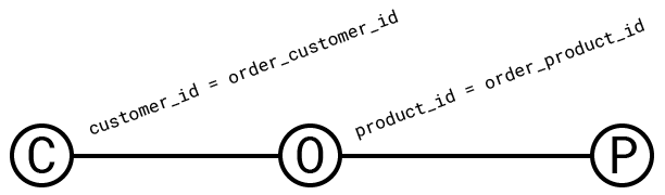
Since a predicate filters the result of the cross product, predicates can be given a numeric value that describes how much they filter said result. This value is called their selectivity. The selectivity of a predicate p on A and B is defined as:

由于谓词过滤叉积的结果，因此可以给谓词一个数值来描述它们过滤所述结果的程度。 这个值称为它们的选择性。 谓词 p 对 A 和 B 的选择性定义为：

sel(p)=∣A×B∣∣A⋈p**B∣=∣A∣∣B∣∣A⋈p**B∣

In practice, we tend to think about this the other way around; we assume that we can estimate the selectivity of a predicate and use that to estimate the size of a join:

在实践中，我们倾向于以相反的方式思考这个问题。 我们假设我们可以估计谓词的选择性并使用它来估计连接的大小：

∣A⋈p**B∣=sel(p)∣A∣∣B∣

So a predicate which filters out half of the rows has selectivity 0.5 and a predicate which only allows one row out of every hundred has selectivity 0.01. Since predicates which are more selective reduce the cardinality of their output more aggressively, a decent general principle is that we want to perform joins over predicates which are very selective first. It’s often assumed for convenience that all the selectivities are independent, that is,

因此，过滤掉一半行的谓词的选择性为 0.5，而仅允许每一百行中的一行的谓词的选择性为 0.01。 由于更具选择性的谓词会更积极地减少其输出的基数，因此一个不错的一般原则是我们希望首先对选择性很强的谓词执行连接。 为了方便起见，通常假设所有选择性都是独立的，即

∣A⋈p**B⋈q**C∣=sel(p)sel(q)∣A×B×C∣

Which, while indeed convenient, is rarely an accurate assumption in practice. Check out “How Good Are Query Optimizers, Really?” by Leis et al. for a detailed discussion of the problems with this assumption.

虽然这确实很方便，但在实践中很少是一个准确的假设。 查看“查询优化器到底有多好？” 莱斯等人。 详细讨论该假设的问题。

It turns out that the shape of a query graph plays a large part in how difficult it is to optimize a query. There are a handful of canonical archetypes of query graph “shapes”, all with different optimization characteristics.

事实证明，查询图的形状在很大程度上决定了优化查询的难度。 有一些查询图“形状”的规范原型，它们都具有不同的优化特征。

​ A “chain” query graph

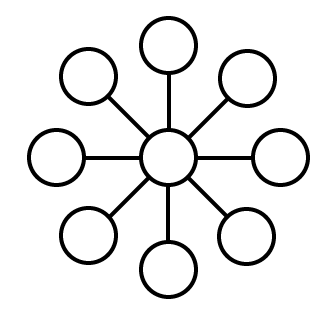
​ A “star” query graph

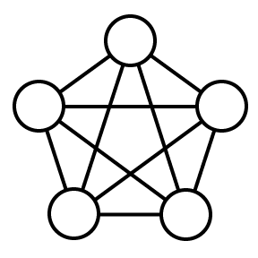
​ A “clique” query graph

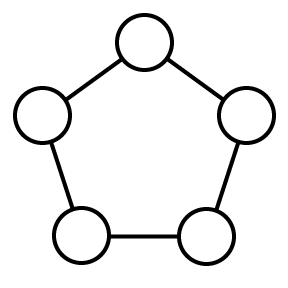
​ A “cycle” query graph

Note that these shapes aren’t necessarily representative of many real queries, but they represent extremes which exhibit interesting behaviour and which permit interesting analysis.

请注意，这些形状不一定代表许多实际查询，但它们代表了表现出有趣行为并允许进行有趣分析的极端情况。

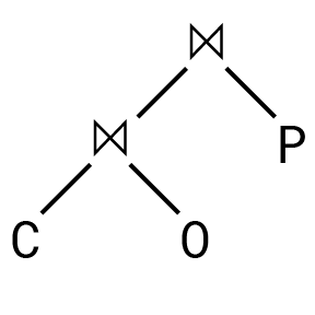
Query Plans

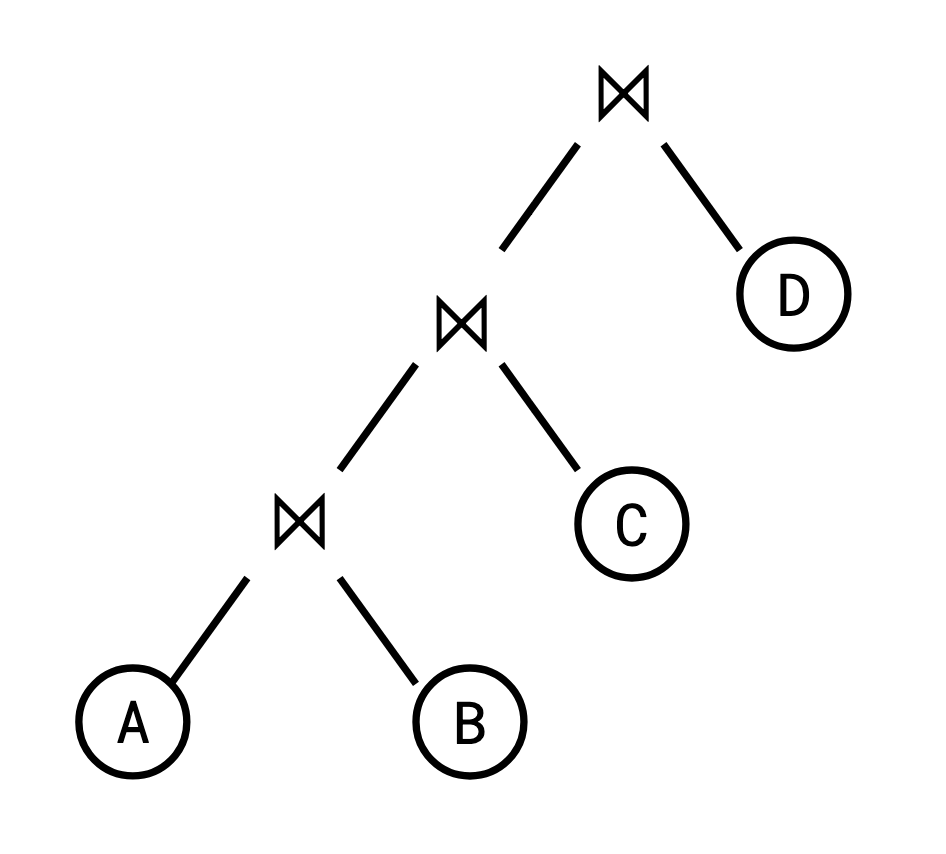
To visualize a particular join ordering, we can look at its query plan diagram. Since most join execution algorithms only perform joins on one pair of relations at a time, these are generally binary trees. The query plan we ended up with for the above query has a diagram that looks something like this:

为了可视化特定的连接顺序，我们可以查看它的查询计划图。 由于大多数连接执行算法一次仅对一对关系执行连接，因此这些通常是二叉树。 我们最终为上述查询得出的查询计划有一个如下所示的图表：

There are also two main canonical query plan shapes, the less general “left-deep plan”:

还有两种主要的规范查询计划形状，即不太通用的“左深度计划”：

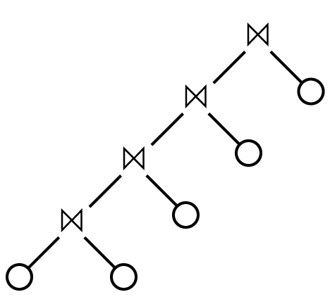
Where every relation is joined in sequence.

每个关系都按顺序连接。

The more general form is the “bushy plan”:

更通用的形式是“bushy plan”：

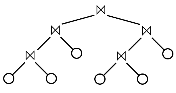
In a left-deep plan, one of the two relations being joined must always be a concrete table, rather than the output of a join. In a bushy plan, such composite inners are permitted.

在左深计划中，连接的两个关系之一必须始终是具体表，而不是连接的输出。 在茂密的规划中，允许使用这种复合材料内部材料。

Is this actually “hard”?

In the examples we’ve seen, there were only a handful of options, but as the number of tables being joined grows, the number of potential query plans grows extremely fast—and in fact, finding the optimal order in which to join a set of tables is NP-hard. This means that when faced with large join ordering problems, databases are generally forced to resort to a collection of heuristics to attempt to find a good execution plan (unless they want to spend more time optimizing than executing!).

在我们看到的示例中，只有少数选项，但随着要连接的表数量的增长，潜在查询计划的数量增长得非常快，事实上，找到连接集合的最佳顺序 表的数量是 NP 困难的。 这意味着，当面临大型连接顺序问题时，数据库通常被迫求助于一系列启发式方法来尝试找到良好的执行计划（除非它们想花更多的时间进行优化而不是执行！）。

I think it’s important to first answer the question of why we need to do this at all. Even if some join orderings are orders of magnitude better than others, why can’t we just find a good order once and then use that in the future? Why does a piece of software like a database that’s concerned with going fast need to solve an NP-hard problem every time it receives a query? It’s a fair question, and there’s probably interesting research to be done in sharing optimization work across queries.

我认为首先回答我们为什么需要这样做的问题很重要。 即使某些连接顺序比其他连接顺序好几个数量级，为什么我们不能一次找到一个好的顺序，然后在将来使用它呢？ 为什么像数据库这样注重速度的软件每次收到查询时都需要解决 NP 难题？ 这是一个公平的问题，在跨查询共享优化工作方面可能需要进行一些有趣的研究。

The main answer, though, is that you’re going to want different join strategies for a query involving Justin Bieber’s twitter followers versus mine. The scale of various relations being joined will vary dramatically depending on the query parameters and the fact is that we just don’t know the problem we’re solving until we receive the query from the user, at which point the query optimizer will need to consult its statistics to make informed guesses about what join strategies will be good. Since these statistics will be very different for a query over Bieber’s followers, the decisions the optimizer ends up making will be different and we probably won’t be able to reuse a result from before.

不过，主要的答案是，对于涉及贾斯汀·比伯 (Justin Bieber) 的 Twitter 关注者和我的关注者的查询，您需要不同的连接策略。 连接的各种关系的规模将根据查询参数的不同而显着变化，事实是，我们只是不知道我们正在解决的问题，直到我们收到用户的查询，此时查询优化器将需要 查阅其统计数据，以做出明智的猜测，了解什么是好的连接策略。 由于对于比伯的关注者的查询，这些统计数据将非常不同，因此优化器最终做出的决策将有所不同，我们可能无法重用之前的结果。

Once you accept that you have to solve the problem, how do you do it? A common characteristic of NP-hard problems is that they’re strikingly non-local. Any type of local reasoning or optimization you attempt to apply to them will generally break down and doom you to look at the entire problem holistically. In the case of join ordering, what this means is that in most cases it’s difficult or impossible to make conclusive statements about how any given pair of relations should be joined - the answer can differ drastically depending on all the tables you don’t happen to be thinking about at this moment.

一旦你承认必须解决问题，你会怎么做？ NP 难问题的一个共同特征是它们明显是非局部的。 您尝试应用于它们的任何类型的局部推理或优化通常都会失败，并注定您必须从整体上看待整个问题。 在连接顺序的情况下，这意味着在大多数情况下，很难或不可能对任何给定的关系对应该如何连接做出结论性的陈述 - 答案可能会有很大不同，具体取决于您没有碰巧的所有表 此刻正在思考。

In our example with customers, orders, and products, it might look like our first plan was bad only because we first performed a join for which we had no predicate (such intermediate joins are just referred to as cross products), but in fact, there are joins for which the ordering that gives the smallest overall cost involves a cross product (exercise for the reader: find one).

在我们的客户、订单和产品示例中，我们的第一个计划可能看起来很糟糕，只是因为我们首先执行了没有谓词的连接（此类中间连接仅称为交叉产品），但事实上， 对于某些连接，给出最小总成本的排序涉及叉积（读者练习：找到一个）。

Despite the fact that optimal plans can contain cross products, it’s very common for query optimizers to assume their inclusion won’t improve the quality of query plans that much, since disallowing them makes the space of query plans much smaller and can make finding decent plans much quicker. This assumption is sometimes called the connectivity heuristic (because it only considers joining relations which are connected in the query graph).

尽管最佳计划可以包含交叉产品，但查询优化器很常见地认为包含它们不会大大提高查询计划的质量，因为不允许它们会使查询计划的空间变得更小，并且可以找到合适的计划 快得多。 这种假设有时称为连接启发式（因为它只考虑查询图中连接的连接关系）。

This post has mostly been about the vocabulary with which to speak and think about the problem of ordering joins, and hasn’t really touched on any concrete algorithms with which to find good query plans.

这篇文章主要是关于谈论和思考连接排序问题的词汇，并没有真正涉及任何用于找到良好查询计划的具体算法。

Join ordering is, generally, quite resistant to simplification. In the general case—and in fact, almost every case in practice—the problem of finding the optimal order in which to perform a join query is NP-hard. However, if we sufficiently restrict the set of queries we look at, and restrict ourselves to certain resulting query plans, there are some useful situations in which we can find an optimal solution. Those details, though, will come in a follow-up post.

一般来说，连接顺序非常难以简化。 在一般情况下（事实上，几乎在实践中的每种情况下），找到执行连接查询的最佳顺序的问题是 NP 困难的。 但是，如果我们充分限制所查看的查询集，并将自己限制为某些结果查询计划，则在某些有用的情况下我们可以找到最佳解决方案。 不过，这些细节将在后续帖子中提供。

If you like this post you can go even deeper on Join Ordering with Join Ordering Part II: The SQL

如果您喜欢这篇文章，您可以通过连接排序第二部分：SQL 更深入地了解连接排序

Join ordering, part II: The ‘SQL’

Even in the 80’s, before Facebook knew everything there was to know about us, we as an industry had vast reams of data we needed to be able to answer questions about. To deal with this, data analysts were starting to flex their JOIN muscles in increasingly creative ways. But back in that day and age, we had neither machine learning nor rooms full of underpaid Excel-proficient interns to save us from problems we didn’t understand; we were on our own.

即使在 80 年代，在 Facebook 了解有关我们的一切之前，我们作为一个行业就拥有大量数据，需要能够回答相关问题。 为了解决这个问题，数据分析师开始以越来越有创意的方式展示他们的 JOIN 力量。 但在那个时代，我们既没有机器学习，也没有满屋子的工资低、精通 Excel 的实习生来帮助我们解决我们不理解的问题； 我们只能靠自己了。

We saw in the previous post how to think about a join ordering problem: as an undirected graph with a vertex for each relation being joined, and an edge for any predicate relating two relations. We also saw the connectivity heuristic, which assumed that we wouldn’t miss many good orderings by restricting ourselves to solutions which didn’t perform cross products.

我们在上一篇文章中看到了如何考虑连接排序问题：作为一个无向图，每个被连接的关系有一个顶点，以及与两个关系相关的任何谓词的边。 我们还看到了连接启发式，它假设通过将自己限制在不执行交叉产品的解决方案中，我们不会错过许多好的订单。

It was discussed that in a general setting, finding the optimal solution to a join ordering problem is NP-hard for almost any meaningful cost model. Given the complexity of the general problem, an interesting question is, how much do we have to restrict ourselves to a specific subclass of problems and solutions to get instances which are not NP-hard?

讨论了在一般情况下，对于几乎任何有意义的成本模型来说，找到连接排序问题的最佳解决方案都是 NP 困难的。 考虑到一般问题的复杂性，一个有趣的问题是，我们必须在多大程度上将自己限制在问题和解决方案的特定子类上才能获得非 NP 困难的实例？

The topic of our story is the IKKBZ algorithm, and the heroes are Toshihide Ibaraki and Tiko Kameda. But first, we need to take a detour through a different field. We will eventually find ourselves back in JOIN-land, so don’t fear, this is still a post about databases.

我们故事的主题是IKKBZ算法，主角是茨木俊秀和龟田提子。 但首先，我们需要绕道进入另一个领域。 我们最终会发现自己回到了 JOIN 领域，所以不要害怕，这仍然是一篇关于数据库的文章。

Maximize Revenue, Minimize Cost 收入最大化，成本最小化

Operations research is a branch of mathematics concerned with the optimization of business decisions and management, and it has led to such developments as asking employees “what would you say you do here?”.

运筹学是数学的一个分支，涉及业务决策和管理的优化，它导致了诸如询问员工“你觉得你在这里做什么？”等发展。

One sub-discipline of operations research is concerned with the somewhat abstract problem of scheduling the order in which jobs in a factory should be performed. For example, if we have some set of tasks that needs to be performed to produce a product, what order will minimize the business’s costs?

运筹学的一个子学科涉及一个有点抽象的问题，即安排工厂中的工作执行顺序。 例如，如果我们需要执行一组任务来生产产品，那么什么顺序可以最大限度地降低企业成本？

The 1979 paper Sequencing with Series-Parallel Precedence Constraints by Clyde Monma and Jeffrey Sidney is interested in a particular type of this problem centered around testing a product for deficiencies. They have a sequence of tests to be performed on the product, some of which must be performed before others. The paper gives the example of recording the payments from a customer before sending out their next bill, in order to prevent double billing - the first task must be performed before the second.

Clyde Monma 和 Jeffrey Sidney 于 1979 年发表的论文《Sequencing with Series-Parallel Precedence Constraints》对这种以测试产品缺陷为中心的特定类型问题感兴趣。 他们要对产品执行一系列测试，其中一些测试必须在其他测试之前执行。 本文给出了在发送下一张账单之前记录客户付款的示例，以防止重复计费 - 第一个任务必须在第二个任务之前执行。

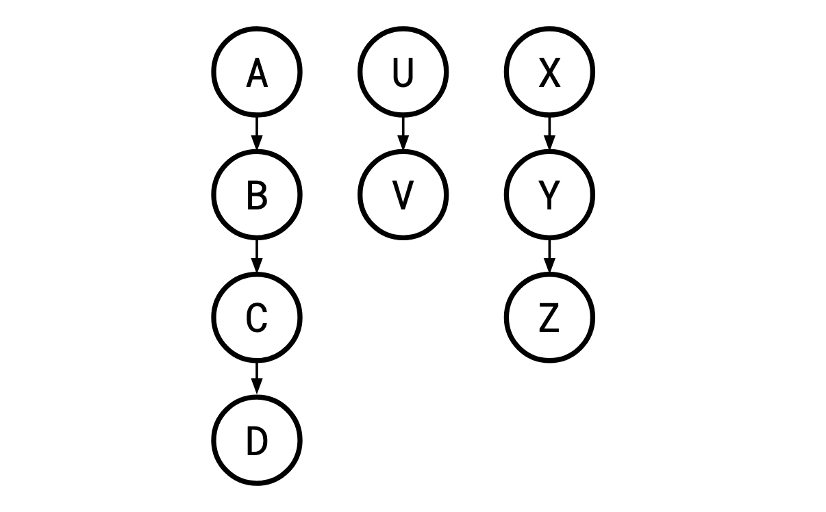
The kind of problem Monma and Sidney cover is one where these tests (henceforth “jobs”) and the order they must be performed in can be laid out in a series of parallel “chains”:

Monma 和 Sidney 所解决的问题是，这些测试（此后称为“作业”）以及它们必须执行的顺序可以布置在一系列并行“链”中：

Where a legal order of the jobs is one in which a job’s parent is carried out before it is, so X,A,B,U,C,V,D,Y,Z is a legal execution here, but A,C,… is not, since B must occur before C. Such restrictions are called sequencing constraints.

如果作业的合法顺序是作业的父作业先于它执行的顺序，则 X,A,B,U,C,V,D, Y,Z 在这里是合法的执行，但 A,C,… 不是，因为 B 必须出现在 C 之前。 此类限制称为排序约束。

This is a specific case of the more general concept of a precedence graph. A precedence graph can just be any directed acyclic graph, so in the general (non-Monma/Sidney) case, such a graph could look like this:

这是更一般的优先级图概念的一个具体情况。 优先图可以是任何有向无环图，因此在一般（非 Monma/Sidney）情况下，这样的图可能如下所示：

In the paper’s setting, each “job” is a test of a component to see if it’s defective or not. If the test fails, the whole process is aborted. If it doesn’t, the process continues. Each test has some fixed probability of failing. Intuitively, the tests we do first should have high probability of detecting a failure, and a low cost: if a test is cheap and has a 99% chance of determining that a component is defective, it would be bad if we did it at the very end of a long, expensive, time-consuming process.

在论文的设置中，每项“工作”都是对一个组件的测试，看看它是否有缺陷。 如果测试失败，则整个过程将中止。 如果没有，该过程将继续。 每个测试都有一些固定的失败概率。 直观上，我们首先进行的测试应该具有很高的检测到故障的概率，并且成本较低：如果测试成本低廉并且有 99% 的机会确定某个组件有缺陷，如果我们在一个漫长、昂贵、耗时的过程的最后才这样做，那就糟糕了。

Next, a job module in a precedence graph is a set of jobs which all have the same relationship to every job not in the module. That is, a set of jobs J is a job module if every job not in J either

接下来，优先级图中的作业模块是一组作业，它们与模块中之外的每个作业都具有相同的关系。 也就是说，如果每个作业都不在 J 中，则一组作业 J 是一个作业模块

1. must come before every job in J, 必须出现在 J 中的每个作业之前，
2. must come after every job in J*, or 必须出现在 J* 中的每项工作之后，或者
3. is unrestricted with respect to every job in J* J*中的每项工作均不受限制

according to the problem’s precedence constraints. 根据问题的优先级约束。

For instance, in this example, {B,C}, {X,Y,Z}, and {V} are job modules, but {X,Z} is not a module because Y must come before Z, but is after X. Similarly, {A,U} is not a module because V must come after U but is unrestricted relative to A.

例如，在此示例中，{B,C}、{X,Y,Z} 和 {V} 是作业模块，但 {X,Z } 不是模块，因为 Y 必须位于 Z 之前，但位于 X 之后。 同样，{A,U} 不是模块，因为 V 必须位于 U 之后，但相对于 A 不受限制。

When we use j to represent an object, we’re talking about one single job, and when we use s and t, we’re talking about strings of jobs, as in, s=j1j2…j**n, which cannot be further split apart, and are performed in sequence. In general, these are somewhat interchangeable. In this setting, jobs are just strings of length one.

当我们使用 j 表示一个对象时，我们谈论的是一个作业，而当我们使用 s 和 t 时，我们谈论的是作业字符串，如 s=j 1j2…j**n，不能再拆分，依次执行。 一般来说，这些在某种程度上是可以互换的。 在这种情况下，作业只是长度为 1 的字符串。

If two strings are in a module together, we can concatenate them in some order to get a new string. Since the constituent jobs and strings are in a module (and thus have all the same constraints), there’s only one natural choice of constraints for this new string to have. It’s generally easier to reason about a problem with fewer jobs in it, so a desirable thing to be able to do is to concatenate two jobs to get a new, simpler problem that is equivalent to the original one. One of the key challenges we’ll face is how to do this.

如果两个字符串一起在一个模块中，我们可以按某种顺序连接它们以获得一个新字符串。 由于组成作业和字符串位于一个模块中（因此具有所有相同的约束），因此这个新字符串只有一种自然的约束选择。 通常，推理作业较少的问题会更容易，因此可以做的一件事是将两个作业连接起来以获得一个与原始问题等效的新的、更简单的问题。 我们将面临的主要挑战之一是如何做到这一点。

We use f(s1,s2,…) to refer to the cost of performing the string s1, followed by the string s2, and so on (think of this function as “flattening” of the sequences of jobs). q(s) is the probability of all of the tests in s succeeding. We assume all the probabilities are independent, and so the probability of all of the jobs in a string succeeding is the product of the probability of success of each individual job. If the sequencing constraints constrain a string s to come before a string t, we write s→t (read “s comes before t”). We’re going to use strings to progressively simplify our problem by concatenating jobs into strings.

我们使用 f(s1,s2,…) 来指代执行字符串 s1、后跟字符串 s2 的成本，依此类推（将此函数视为 工作序列的“扁平化”）。 q(s) 是 s 中所有测试成功的概率。 我们假设所有概率都是独立的，因此字符串中所有作业成功的概率是每个作业成功概率的乘积。 如果排序约束将字符串 s 限制在字符串 t 之前，则我们编写 s→t （读作“s 在 t 之前”）。 我们将使用字符串通过将作业连接到字符串中来逐步简化我们的问题。

The expected cost of performing one sequence of jobs followed by another sequence of jobs is the cost of performing the first sequence plus the cost of performing the second sequence, but we only have to actually perform the second sequence if the first sequence didn’t fail. Thus, in expectation, the cost is f(s,t)=f(s)+q(s)f(t).

执行一个作业序列，然后执行另一个作业序列的预期成本是执行第一个序列的成本加上执行第二个序列的成本，但如果第一个序列没有失败，我们只需实际执行第二个序列 。 因此，预计成本为 f(s,t)=f(s)+q(s)f(t)。

Since this is recursive, we need a base case, and of course, the cost of performing a single job is simply the cost of the job itself: f(j)=c**j. An important property of this definition is that f is well-defined: f(S1,S2)=f(S1′,S2′) whenever ′S1S2=S1′S2′ (verifying this is left as an exercise).

由于这是递归的，我们需要一个基本情况，当然，执行单个作业的成本就是作业本身的成本：f(j)=c**j。 该定义的一个重要属性是 f 是明确定义的：f(S1,S2)=f(S1′,S2′) 每当 ′* S1S2=S1′S*2′（验证这一点留作练习）。

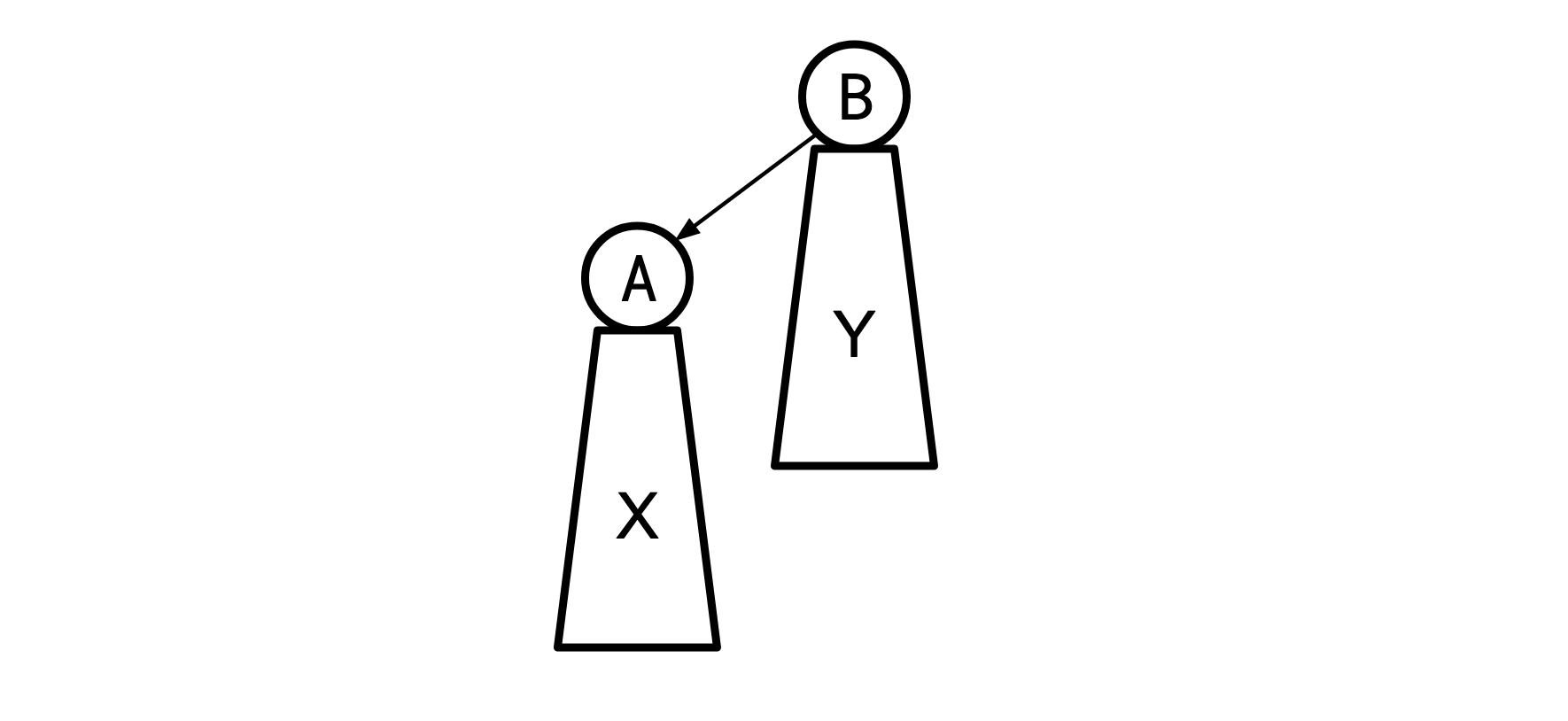
An adjacent sequence interchange is a swap of two adjacent sequences within a larger sequence:

相邻序列互换是一个较大序列内两个相邻序列的交换：

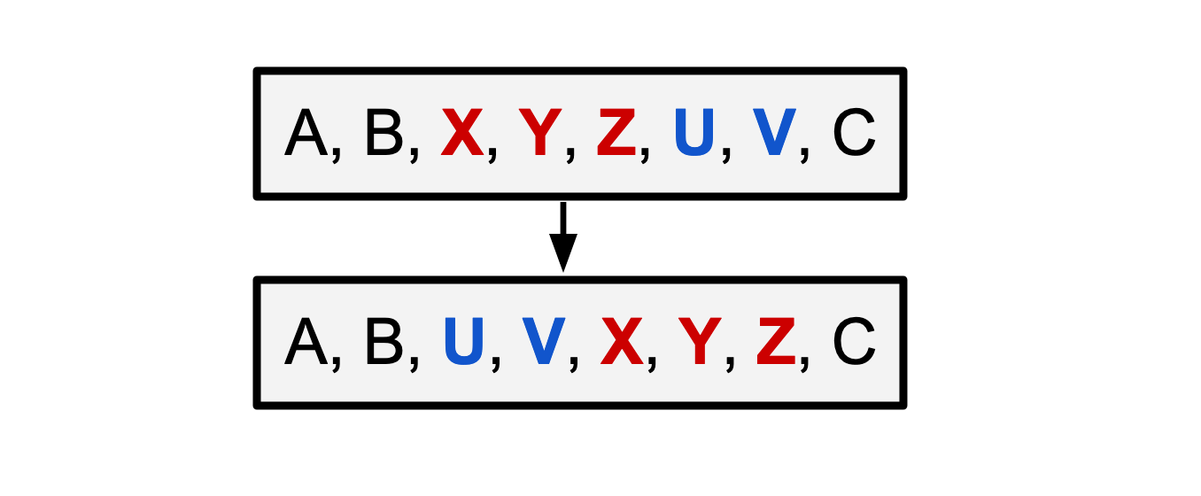
This is an adjacent sequence interchange of X,Y,Z with U*,V.

这是 X、Y、Z 与 U、V* 的相邻序列互换。

A rank function maps a sequence of jobs j1j2…jn to a number. Roughly, a rank function captures how desirable it is to do a given sequence of jobs early. r(s)<r(t) means we would like to do s before t. A cost function is called adjacent sequence interchange (ASI) relative to a rank function r if the rank function accurately tells us when we want to perform interchanges:

排名函数 将作业序列 j1j2…jn 映射到一个数字。 粗略地说，排名函数反映了尽早完成给定工作序列的期望程度。 r(s)<r(t) 意味着我们想在 t 之前执行 s。 如果排名函数准确地告诉我们何时要执行交换，则相对于排名函数r，成本函数被称为相邻序列交换（ASI）：

f(a,s,t,b)≤f(a,t,s,b) if r(s)≤r(t)

And a cost function f is ASI if there exists a rank function it is ASI relative to. I’m sure you’ll be shocked to learn the f we derived above f*(s,t)=f(s)+q(s)f(t)) is ASI.

如果存在相对于 ASI 的排序函数，则成本函数 f 就是 ASI。 我相信您会惊讶地发现我们上面推导出的 f f*(s,t)=f(s)+q(s)f (t)) 是 ASI。

Note that even though we may have a rank function which tells us we would like to do a given sequence of jobs early, the sequencing constraints might prohibit us from doing so.

请注意，即使我们可能有一个排名函数告诉我们希望尽早执行给定的作业序列，但排序约束可能会阻止我们这样做。

The ASI theorem (Monma and Sidney call this “Theorem 2”, but we’re going to use it enough for a real name) mildly paraphrased:

ASI 定理（Monma 和 Sidney 称之为“定理 2”，但我们将用它来表示真实的名字）温和地解释道：

​ Let *f be ASI with rank function r, and let *s* and *t* be strings. Consider a job module {*s*,*t*} in a general precedence graph, where *s→*t and *r*(*t*)≤*r*(*s*). Then there is an optimal permutation with *s* immediately preceding *t*.*

令*f 为具有排名函数r 的ASI，并令*s* 和*t* 为字符串。 考虑一般优先级图中的作业模块 {*s*,*t*}，其中 *s→*t 且 *r*(*t*)≤*r*(* s*)。 然后有一个最佳排列，其中 *s* 紧接在 *t*.* 之前

Let’s break down this theorem. First of all, note that it applies to a *general* precedence graph. This means we’re not restricting ourselves to the “parallel chains” kind of graph described above.

让我们来分解一下这个定理。 首先，请注意，它适用于一般优先级图。 这意味着我们不会将自己限制在上述“平行链”类型的图表中。

s→t means s must come before t* (s and t are already strings in the current iteration of our problem, and they inherit the constraints of the jobs they are composed of). However, )r(t)≤r(s) means we would like to put t before s. What this theorem is saying is that in this scenario, we’re not forgoing optimality by ordering s immediately before t. This is very useful, because it allows us to take two strings, s and t, and replace them with the new string s**t which is their concatenation. Importantly, this is saying that there is an optimal permutation with s immediately preceding t, not that in any every optimal permutation this is the case. The proof of this theorem is pretty simple so I’ve included it.

s→t 意味着 s 必须在 t* 之前（s 和 t 在我们问题的当前迭代中已经是字符串，并且它们继承了它们所组成的作业的约束）。 然而，r(t)≤r(s) 意味着我们喜欢将t放在s之前。 该定理的意思是，在这种情况下，我们不会通过在 t 之前立即排序 s 来放弃最优性。 这非常有用，因为它允许我们获取两个字符串 s 和 t，并将它们替换为新字符串 s**t（它们的串联）。 重要的是，这意味着存在一个最优排列，其中s紧接在t之前，而不是在任何每个最优排列中都是这种情况。 这个定理的证明非常简单，所以我把它包括在内。

Proof of the ASI theorem:
Every optimal permutation looks like ⟨u,s,v,t,w⟩ since s→t*. If v is empty, we’re done. otherwise, if r*(v)≤r(s), then by ASI we can swap s and v without dropping the cost to get ⟨u,v,s,t,w⟩. If r*(s)<r(v), then by transitivity r(t)<r(v) and again by ASI we can swap v and t without dropping the cost to get ⟨u,s,t,v,w⟩. These swaps must be legal since {s,t} is a job module.

每个最优排列看起来都像 ⟨u,s,v,t,w⟩，因为 s→t。 如果 v 为空，我们就完成了。 否则，如果 r(v)≤r(s)，那么通过 ASI 我们可以交换 s 和 v 而不会降低得到 ⟨u,v,s 的成本 ，t，w⟩。 如果 r*(s)<r(v)，则通过传递性 r(t)<r(v) 并再次通过 ASI，我们可以交换 v 和 * t，而不降低获得 ⟨u*,s,t,v,w⟩ 的成本。 这些交换必须是合法的，因为 {s,t} 是一个作业模块。

Finally, our friends Monma and Sidney describe the parallel chains algorithm. It goes like this:

最后，我们的朋友 Monma 和 Sidney 描述了平行链算法。 事情是这样的：

1. If, for every pair of strings �⃗s and �⃗t, �⃗→�⃗s→t implies �(�⃗)<�(�⃗)r(s)<r(t) (meaning that the constraints and the rank agree about the correct order for the two), go on to step 2. If the two relations disagree somewhere, then we can find a job module {�⃗,�⃗}{s,t} for which they disagree [1]. Then, by the ASI theorem, we can concatenate �⃗s and �⃗t into the sequence �⃗�⃗s**t (since we know there’s some optimal solution where they’re adjacent), which we then treat as a new string. Now repeat step 1. Our problem has exactly one less string in it now, so this process can’t go on forever.
2. Sort the remaining strings by their value under �r. Since step 1 terminated, the resulting order is legal, and since �f is ASI, it’s optimal.

The core idea of the algorithm is that we’d like to just blindly order all the jobs by their value under the rank function, but situations where the rank function and the precedence constraints disagree prohibit that. The ASI theorem gives us a tool to eliminate precisely these scenarios while keeping access to optimal solutions, so we repeatedly apply it until we are free to simply sort.

该算法的核心思想是，我们希望按照排名函数下的值对所有作业进行盲目排序，但排名函数和优先级约束不一致的情况会禁止这样做。 ASI 定理为我们提供了一个工具，可以精确消除这些情况，同时保持获得最佳解决方案的能力，因此我们反复应用它，直到我们可以自由地进行简单排序。

Back to Databases

Back to the topic of Join Ordering. For their paper “On the Optimal Nesting Order for Computing N-Relational Joins,” Toshihide Ibaraki and Tiko Kameda were interested in instances of the join ordering problem for which

回到连接排序的主题。 Toshihide Ibaraki 和 Tiko Kameda 在他们的论文“On the Optimal Nesting Order forComputing N-Relational Joins”中对连接排序问题的实例感兴趣，其中

• solutions were restricted to those that 解决方案仅限于那些
  • were left-deep and 是左深和
  • contained no cross products 不包含交叉产品
• the only join algorithm used was the nested-loop join, and 使用的唯一连接算法是嵌套循环连接，并且
• the query graph was a tree. 查询图是一棵树。

As we saw before, a plan is left-deep if the right input to every join operator is a concrete relation, and not another join operation. This gives a query plan that looks something like this, with every right child being a “base relation” and not a join:

正如我们之前所看到的，如果每个连接运算符的右侧输入是具体关系，而不是另一个连接操作，则计划是左深的。 这给出了一个看起来像这样的查询计划，其中每个右子节点都是“基本关系”而不是联接：

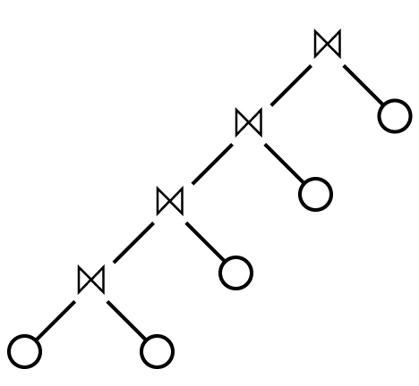
and not like this, where a join’s right child can be another join: 而不是这样，一个连接的右子节点可以是另一个连接：

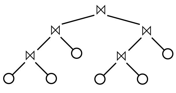
Since the shape of the plan is fixed, we can talk about the plan itself simply as a sequence of the relations to be joined, from left to right in the left-deep tree. We can take a query plan like this:

由于计划的形状是固定的，因此我们可以将计划本身简单地视为要连接的关系序列，在左深树中从左到右。 我们可以采用这样的查询计划：

and represent it like this: 并像这样表示它：

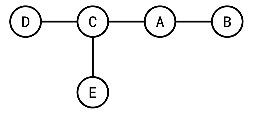
When we say that the query graph must be a “tree”, we mean in a graph theoretical sense—it’s a graph that is connected and has no cycles. If you primarily identify as a computer science person and not a mathematician, when you hear “tree” you might picture what graph theorists call a “rooted” tree. That is, a tree with a designated “special” root vertex. It’s like you grabbed the tree by that one designated vertex and let everything else hang down.

当我们说查询图必须是一棵“树”时，我们指的是图论意义上的——它是一个连通且没有环的图。 如果您主要认为自己是计算机科学家而不是数学家，那么当您听到“树”时，您可能会想到图论学家所说的“有根”树。 也就是说，一棵树具有指定的“特殊”根顶点。 这就像你抓住了树的一个指定顶点，然后让其他所有东西都垂下来。

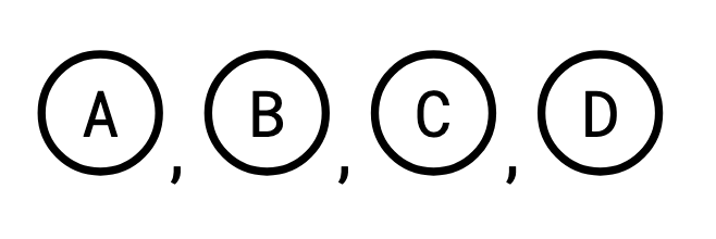
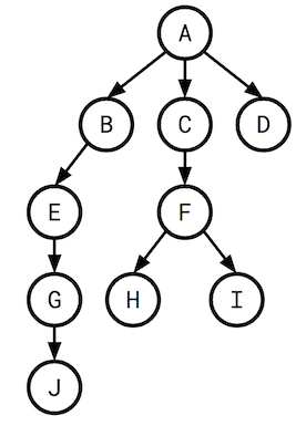
Here’s a tree:

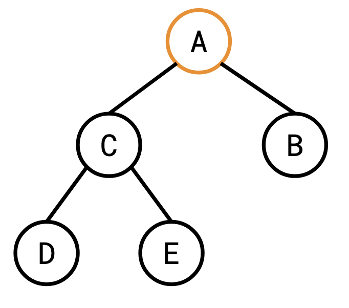
Here it is rooted at �A:

Here it is rooted at �D:

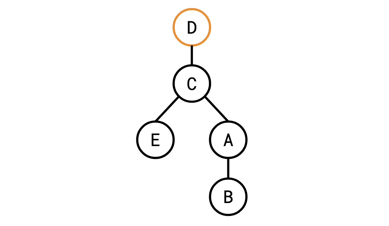
This distinction is important for our purposes because it’s easy to get a rooted tree from an unrooted tree: you just pick your favourite vertex and call it the root.

这种区别对于我们的目的很重要，因为很容易从无根树中获得有根树：您只需选择您最喜欢的顶点并将其称为根即可。

Query graphs and query plans are fundamentally different. The query graph describes the problem and a query plan the solution. Despite this, they’re related in very important ways. In a left-deep query plan, the relation in the bottom-left position is quite special: it’s the only one which is the left input to a join. If we are obeying the connectivity heuristic (no cross products), this gives us a way to think about how exactly it is we are restricted.

查询图和查询计划有着根本的不同。 查询图描述了问题，查询计划描述了解决方案。 尽管如此，它们在非常重要的方面是相关的。 在左深查询计划中，左下位置的关系非常特殊：它是唯一一个连接的左输入。 如果我们遵循连通性启发式（无交叉乘积），这将给我们一种思考我们到底受到怎样的限制的方法。

In the plan above, A and B must share a predicate, or else they would cross-product with each other. Then C must share a predicate with at least one of A or B. Then D must share a predicate with at least one of A, B, or C, and so on.

在上面的计划中，A 和 B 必须共享一个谓词，否则它们将相互交叉积。 那么C 必须与A 或B 中的至少一个共享谓词。 那么D 必须与A、B 或C 等中的至少一个共享谓词。

Let’s assume for a second that given a query graph, we know which relation will wind up in the bottom-left position of an optimal plan. If we take this special relation and make it the root in our query graph, something very useful happens.

让我们假设给定一个查询图，我们知道哪个关系将出现在最佳计划的左下角位置。 如果我们采用这种特殊关系并将其作为查询图中的根，就会发生一些非常有用的事情。

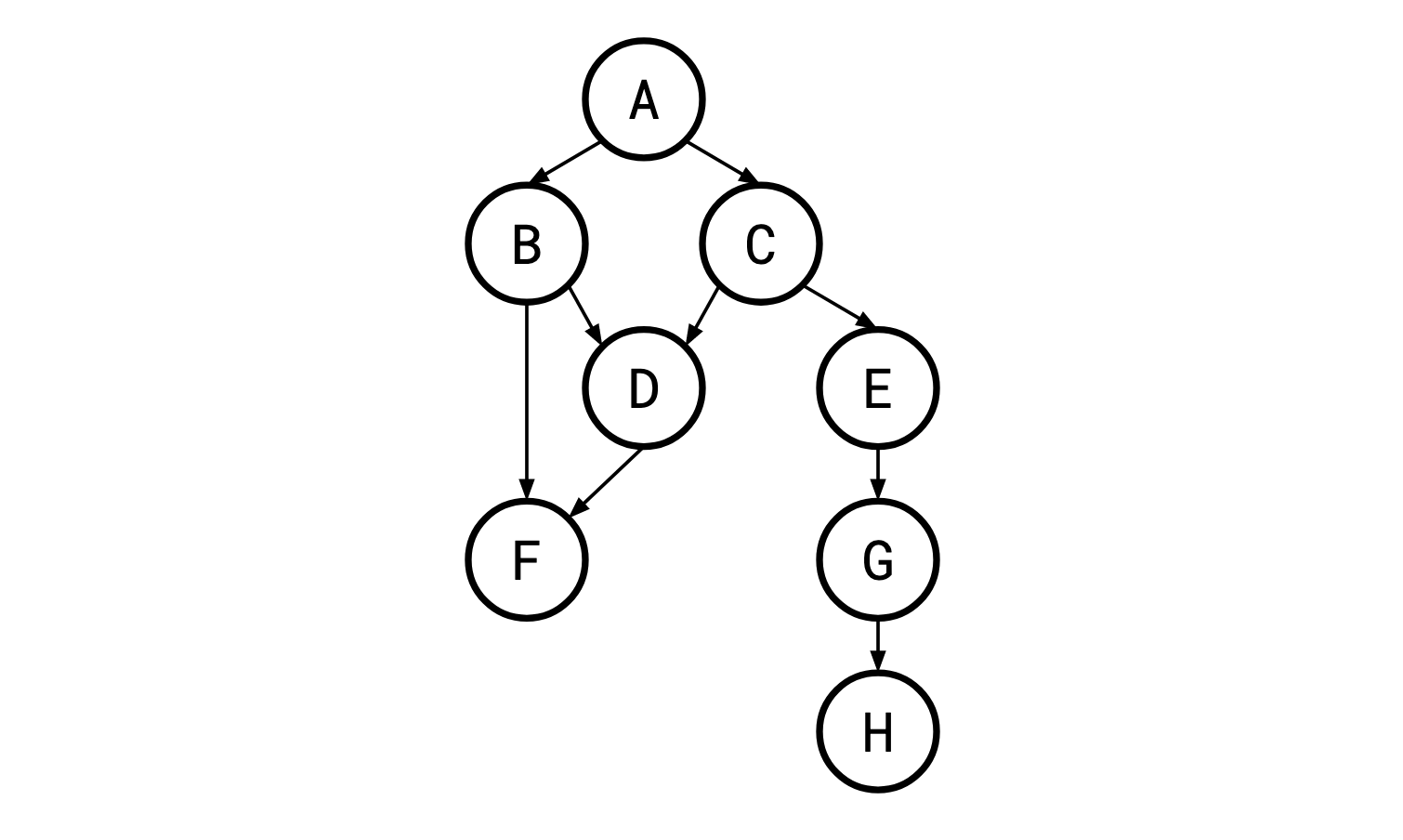
Given our rooted query graph, let’s figure out what a plan containing no cross products looks like. Here’s an example of such a rooted query graph:

给定我们的根查询图，让我们弄清楚不包含叉积的计划是什么样子的。 这是此类有根查询图的示例：

Since we must lead with A, which vertices can we then add to get a legal ordering? Well, the only three that don’t form a cross product with A are B, C, and D. Once we output, C, it becomes legal to output F*, and so on. As we go down the tree, we see a necessary and sufficient condition for not introducing cross products is that the parent of a given relation must have already been output. This is effectively the same as the precedence constraints of the job-scheduling problem!

既然我们必须以 A 开头，那么我们可以添加哪些顶点来获得合法的排序？ 好吧，唯一不与 A 形成叉积的三个是 B、C 和 D。 一旦我们输出C，输出F*就变得合法，依此类推。 当我们沿着树往下走时，我们看到不引入叉积的充分必要条件是给定关系的父关系必须已经输出。 这实际上与作业调度问题的优先级约束相同！

Of course, beforehand, we don’t know which relation will be the optimal one to place in the bottom left. This is going to turn out to be only a minor problem: we can just try each possible relation and choose the one that gives us the best result.

当然，事先我们“不”知道哪一种关系最适合放置在左下角。 这将只是一个小问题：我们可以尝试每种可能的关系并选择给我们最好结果的关系。

So, from here on, we’ll think of our query graph as a rooted tree, and the root will be the very first relation in our join sequence. Despite our original graph having undirected edges, this choice allows us to designate a canonical direction for our edges: we say they point away from the root.

因此，从现在开始，我们将查询图视为一棵有根树，根将是连接序列中的第一个关系。 尽管我们的原始图具有无向边，但这种选择允许我们为边指定规范方向：我们说它们指向远离根的方向。

A Tale of Two Disciplines 两个学科的故事

I can only imagine that what happened next went something like this:

我只能想象接下来发生的事情是这样的：

Kameda sips his coffee as he ponders the problem of join ordering. He and Ibaraki have been collaborating on this one for quite a while, but it’s a tough nut to crack. The data querying needs of industry grow ever greater, and he has to deliver to them a solution. He decides to take a stroll of the grounds of Simon Fraser University to clear his mind. As he locks his office, his attention is drawn by the shuffling of paper. A postdoc from the operations research department is hurrying down the hall, an armful of papers from the past few years tucked under her arm.

龟田一边喝着咖啡，一边思考加入点菜的问题。 他和茨木在这个问题上已经合作了一段时间，但这是一个很难解决的问题。 行业的数据查询需求越来越大，他必须给他们提供一个解决方案。 他决定在西蒙弗雷泽大学的校园里漫步，以理清思绪。 当他锁上办公室时，他的注意力被翻动的纸张吸引了。 一名运筹学系的博士后正匆匆走过大厅，腋下夹着一摞过去几年的论文。

Unnoticed, one neatly stapled bundle of papers drops to the floor from the postdoc’s arm. “Oh, excuse me! You dropped—” Kameda’s eyes are drawn to the title of the paper, Sequencing With Series-Parallel Precedence Constraints, as he bends down to pick it up.

不知不觉中，一叠装订整齐的论文从博士后的手臂上掉到了地板上。 “哦，对不起！ 你掉下来了——”龟田弯下腰捡起它时，他的眼睛被论文的标题《具有系列并行优先约束的测序》所吸引。

“Oh, thank you! I never would have noticed,” the postdoc says, as she turns around and reaches out a hand to take back the paper. But Kameda can no longer hear her. He’s entranced. He’s furiously flipping through the paper. This is it. This is the solution to his problem. The postdoc stares with wide eyes at his fervor. “I…I’ll return this to you!” He stammers, as he rushes back to his office to contact his longtime collaborator Ibaraki.

“哦谢谢！ 我永远不会注意到，”博士后说，她转身伸出手拿回论文。 但龟田已经听不到她的声音了。 他很着迷。 他正在疯狂地翻阅报纸。 就是这个。 这就是他的问题的解决方案。 博士后睁大眼睛盯着他的热情。 “我……我会把这个还给你！” 他结结巴巴地冲回办公室联系他的长期合作者茨木。

If this isn’t how it happened, I’m not sure how Ibaraki and Kameda ever made the connection they did, drawing from research about a problem in an entirely different field from theirs. As we’ll see, we can twist the join ordering problem we’re faced with to look very similar to a Monma-and-Sidney job scheduling problem.

如果事情不是这样发生的，我不确定茨城和龟田是如何从与他们完全不同领域的问题的研究中建立起这种联系的。 正如我们将看到的，我们可以将面临的连接排序问题扭曲成与 Monma-and-Sidney 作业调度问题非常相似。

Recall that the selectivity of a predicate (edge) is the amount that it filters the join of the two relations (edges) it connects (basically, how much smaller its result is than the raw cross product):

回想一下，谓词（边）的选择性是它过滤它连接的两个关系（边）的连接的量（基本上，它的结果比原始叉积小多少）：

sel(p)=∣A×B∣∣A⋈p**B∣

Designating a root allows us another convenience: before now, when selectivity was a property of a predicate, we had to specify a pair of relations in order to say what their selectivity was. Now that we’ve directed our edges, we can define a selectivity for a given relation (vertex) as the selectivity of it with its parent, with the selectivity of the root being defined as 1. So in our graph above, we define the selectivity of H to be the selectivity of the edge between F and H. We refer to the selectivity of R* by f**R.

指定根为我们提供了另一个便利：以前，当选择性是谓词的属性时，我们必须指定一对关系才能说明它们的选择性是什么。 现在我们已经确定了边的方向，我们可以将给定关系（顶点）的选择性定义为其与其父级的选择性，根的选择性定义为 1。因此，在上图中，我们 将* H 的选择性定义为F* 和H 之间边缘的选择性。 我们用 f**R 来表示 R* 的选择性。

This definition is even more convenient than it first appears; we’re restricted by the precedence constraints already to include the parent of a relation before the relation itself in any legal sequence, thus, by the time a relation appears in the sequence, the predicate from which it derives its selectivity will apply. This allows us to define a very simple function which captures the expected number of rows in a sequence of joins. Let ∣N**i=∣R**i∣, then for some sequence of relations to be joined S, let T(S) be the number of rows in the result of evaluating S. Then:

这个定义比乍一看更加方便； 我们已经受到优先约束的限制，在任何合法序列中都必须在关系本身之前包含关系的父关系，因此，当关系出现在序列中时，将应用从中得出其选择性的谓词。 这允许我们定义一个非常简单的函数，它捕获连接序列中的预期行数。 令∣N**i=∣R**i∣，然后对于要连接S的某些关系序列，令T(S)为评估结果中的行数 S。 然后：

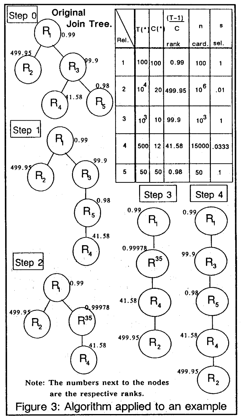
There’s one final piece to fall into place to get the final IKKBZ algorithm. The IK in IKKBZ indeed stands for Ibaraki and Kameda. At VLDB 1986, Ravi Krishnamurthy, Haran Boral, and Carlo Zaniolo presented their paper Optimization of Nonrecursive Queries. Check out this glorious 1986-era technical diagram from their paper:

为了获得最终的 IKKBZ 算法，还需要完成最后一项工作。 IKKBZ中的IK确实代表茨城和龟田。 在 VLDB 1986 上，Ravi Krishnamurthy、Haran Boral 和 Carlo Zaniolo 发表了他们的论文“非递归查询的优化”。 看看他们论文中这张 1986 年时代的技术图表：

Their trick is that if we pick A as our root and find the optimal solution from it, and then for our next choice of root we pick a vertex B that is adjacent to A, a lot of the work we’ll have to do to solve from B will be the same as the work done from A.

他们的技巧是，如果我们选择 A 作为我们的根并从中找到最佳解决方案，然后对于我们下一个选择的根，我们选择一个与 A 相邻的顶点 B，我们需要做很多工作。 从 B 解决所需的工作将与从 A 完成的工作相同。

Consider a tree rooted at A:

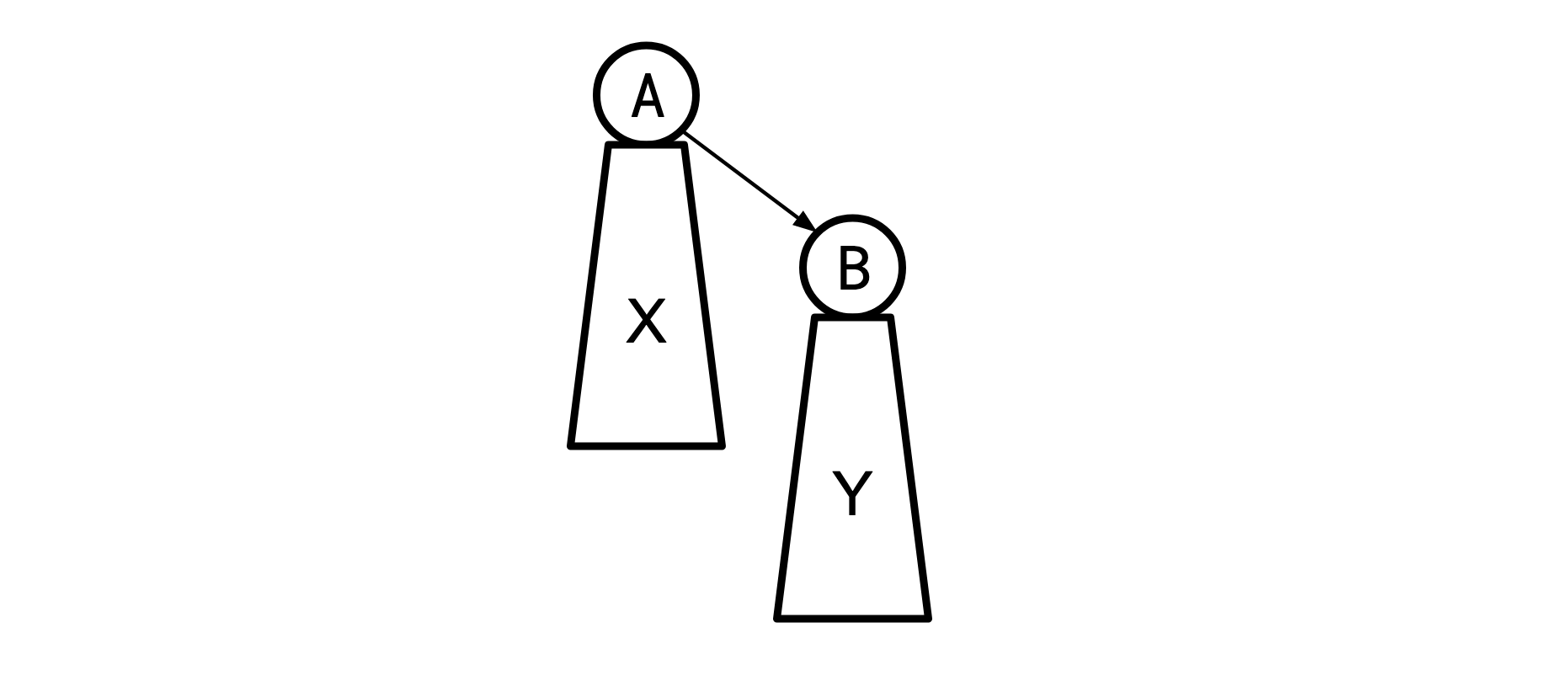
(Where X is all the nodes that live beneath A and Y is all the nodes that live beneath B) and say we have the optimal solution S for the A tree. We then we re-root to B:

（其中 X 是位于 A 下的所有节点，Y 是位于 B 下的所有节点）并说我们有 A 树的最佳解决方案 S。 然后我们重新root到B：

KB&Z recognized that the X and Y subtrees in these two cases are the same, and thus when we eliminate all the wedges beneath A and B, the resulting chains will be in the same order they were in for the tree rooted at A, and this order is the same as the order implied by S. So we can turn the X* and Y subtrees into chains by just sorting them by the order they appear in S.

KB&Z 认识到这两种情况下的 X 和 Y 子树是相同的，因此当我们消除 A 和 B 下面的所有楔子时，生成的链将采用与它们原来的顺序相同的顺序 以 A 为根的树，并且 此顺序与 S 隐含的顺序相同。 因此，我们只需按照它们在 S 中出现的顺序对它们进行排序，就可以将 X* 和 Y 子树变成链。

This means that we can construct the final chains beneath A* and B* without a O(nlogn) walk, using only O(n) time to merge the two chains, so in aggregate, we do this for every choice of root, and arrive at a final runtime of O(n2).

这意味着我们可以在 A* 和 B* 下面构建最终的链，而无需 O(nlogn) 步，仅使用 O(n) 时间来合并两个链，因此 总的来说，我们对每个根选择都执行此操作，并达到 O(n2) 的最终运行时间。

OK, let’s take a step back. Who cares? What’s the point of this algorithm when the case it handles is so specific? The set of preconditions for us to be able to use IKKBZ to get an optimal solution was a mile long. Many query graphs are not trees, and many queries require a bushy join tree for the optimal solution.

好吧，让我们退一步。 谁在乎？ 当这个算法处理的案例如此具体时，它还有什么意义呢？ 我们能够使用 IKKBZ 获得最佳解决方案的先决条件有一英里长。 许多查询图不是树，并且许多查询需要茂密的连接树才能获得最佳解决方案。

What if we didn’t rely on IKKBZ for an optimal solution? Some more general heuristic algorithms for finding good join orders require an initial solution as a “jumping-off point.” When using one of these algorithms, IKKBZ can be used to find a decent initial solution. While this algorithm only has guarantees when the query graph is a tree, we can turn any connected graph into a tree by selectively deleting edges from it (for instance, taking the min-cost spanning tree is a reasonable heuristic here).

如果我们不依赖 IKKBZ 来获得最佳解决方案怎么办？ 一些用于寻找良好连接顺序的更通用的启发式算法需要一个初始解决方案作为“起点”。 当使用其中一种算法时，IKKBZ 可用于找到合适的初始解决方案。 虽然该算法仅在查询图是树时有保证，但我们可以通过有选择地删除其中的边来将任何连通图转换为树（例如，采用最小成本生成树在这里是一个合理的启发式）。

The IKKBZ algorithm is one of the oldest join ordering algorithms in the literature, and it remains one of the few polynomial-time algorithms that has strong guarantees. It manages to accomplish this by being extremely restricted in the set of problems it can handle. Despite these restrictions, it can still be useful as a stepping stone in a larger algorithm. Adaptive Optimization of Very Large Join Queries has an example of an algorithm that makes use of an IKKBZ ordering as a jumping off point, with good empirical results. CockroachDB doesn’t use IKKBZ in its query planning today, but it’s something we’re interested in looking into in the future.

IKKBZ 算法是文献中最古老的连接排序算法之一，并且它仍然是少数具有强有力保证的多项式时间算法之一。 它通过严格限制它可以处理的问题来实现这一目标。 尽管有这些限制，它仍然可以作为更大算法的垫脚石。 超大型连接查询的自适应优化有一个算法示例，该算法使用 IKKBZ 排序作为起点，具有良好的经验结果。 目前，CockroachDB 在其查询规划中并未使用 IKKBZ，但我们将来有兴趣研究它。

Sketch of a proof of [1]:
Since the two are related by the precedence constraints, they’re in the same chain. If they’re not adjacent in that chain, there’s some �x in between them, so �⃗→�⃗→�⃗s→x→t. If �(�⃗)<�(�⃗)r(x)<r(t), then {�⃗,�⃗}{x,t} is a “closer” bad pair. If �(�⃗)≥�(�⃗)r(x)≥r(t) then {�⃗,�⃗}{x,s} is a “closer” bad pair. Then by induction there’s an adjacent pair.